When having to work with a long datasheet in Excel, if you don’t color row alternately, the probability of making mistakes will be very high. The following article will guide you through this technique easily and help the list in your datasheet clearer.
Step 1: Open Excel datasheet
Step 2: Color rows on datasheet alternately
On the program’s interface, you go to Home tag of Ribbon bar, select Conditional Formatting in Style group, and then select New Rule in the drop-down menu.
Step 2: Color rows on datasheet alternately
On the program’s interface, you go to Home tag of Ribbon bar, select Conditional Formatting in Style group, and then select New Rule in the drop-down menu.

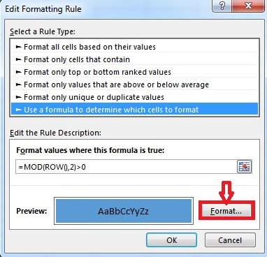
At that time, New Formatting Rule dialogue box occurs, at cell Format values where this formula is true, you type the following formula: =MOD(ROW(),2)>0

Afterward, to select color for rows alternately, you click Format, Format Cells dialogue box occurs, select Fill tab and select color (here, betdownload.com choose light green color). Finally, press OK to complete.

Step 3: Change color on alternate rows
If you want to select other colors (different from the above light green color), select Conditional Formatting and then clickManage Rule.
If you want to select other colors (different from the above light green color), select Conditional Formatting and then clickManage Rule.

Conditional Formatting Rule Manager dialogue box occurs, you select Edit Rule.

Click Format cell and reselect the color that you want to change (here, betdownload.com select yellow color), the click OKto complete.
Results have been changed:

Wish you success!


Post a Comment